Post 101 - Entry Test for MBDyn

Step 1: First contact

The first step aims to evaluate if we were successfully able to download, compile, create a test and finally run it. Therefore, I started by downloading the current MBDyn version from Software Download page.

In order to install MBDyn, I executed the following commands:

mkdir mbdyn-1.7.3
tar -zvxf mbdyn-1.7.3.tar.gz -C mbdyn-1.7.3
./configure
make
make check
make install

The installation was successful; however, since the MBDyn had been installed at /usr/local/mbdyn/bin, I needed to add this diretory path to the system by editing the .bashrc .file. The following line of code was added:

export PATH=${PATH}:/usr/local/mbdyn/bin/

Example Test:

In order to test if the tool was working correctly, a Hello World script was evaluated. I extracted it from Sky Engineering Laboratory Inc. There are several examples about how to simulate mechanical systems, as well as tutorials and simulations. I chose the Double Rigid Pendulum which can also be found here as well.

Then, run the following command:

mbdyn -f double_rigid_pendulum.mbd

The simulation was executed with success and I noted it created 5 other files with the same name; however, with different extensions. The data is stored in the files .ine and .mov, which correspond to the kinematic and dynamic output data.

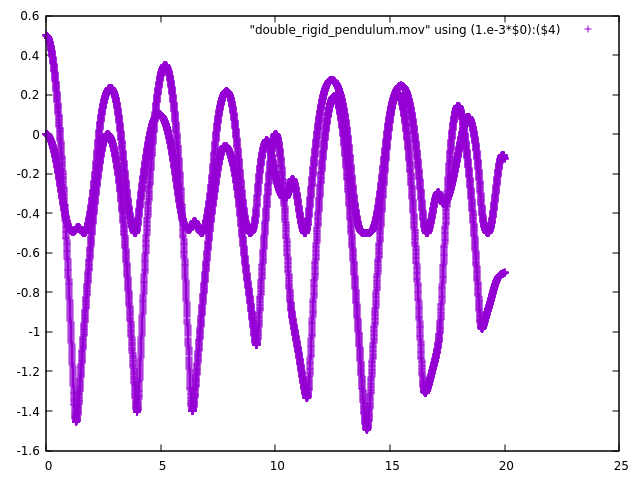
The first way of plotting the movement of the rigid body is by using gnuplot:

gnuplot
plot "double_rigid_pendulum .mov" using (1.e-3*$0):($4)

The following picture illustrates the results using gnuplot:

Another approach to display the output is using Matlab. Probably, there is some code on MBDyn website which already extracts the normalized data into matlab. I created a script which can store the output data into variables. Also, for this example, I created the following simulation:

Step 2: Developing a branch of MBDyn main repository

So far, I was able to install the latest version of MBDyn, which is version 1.7 and play around with mbdyn codes. In order to see the result of a simulation, I used gnuplot in the command line and Matlab as I already showed.

For step 2, it is asked to implement a modification to the MBDyn code used for step 1 and then re-run step 1. In order to do it, I donwloaded and compiled the most recent source code at GitLab.

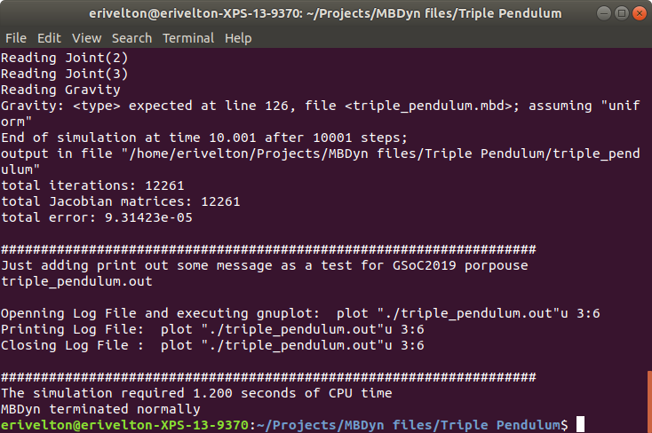
The MBDyn does not provide a graphical interface and I could not find any command to plot the outputs. I just noticed it generates the output as already mentioned. Therefore, one of the future modifications is to add a functionlity to plot the results directly from the mbdyn tool. In order to evaluate the use of ploting tools on source code, I used gnuplot inside of MBDyn. The goal here is to plot one of the output files sInputFileName.out. This file is depicted in the following figure:

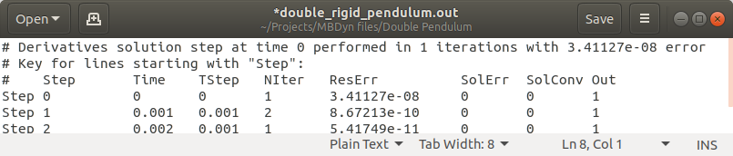
The modification proposed consist of the plot ResErr versus Simulation Time. The same concept could be use to plot kinematic and dynamic results. The modified files to perform this task were:

• solver.cc
• solver.h

Somehow, I was not able to fork the repository to be able to pull my modifications. I believe I need permission to fork this repository. To mitigate it, I created a repositoy at my github account and uploaded all the modified code and other codes I used in this post. To download the repository execute the following from the command line:

git clone git@github.com:EriveltonGualter/GSoC-MBDyn.git

or download directly here: https://github.com/EriveltonGualter/GSoC-MBDyn

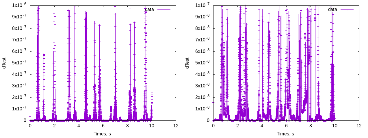
Therefore, after re-running the code, a plot will be created in the same directory of the output files. The following figures were generated by this new source code for the previous mbdyn code, where the left corresponds to the results for double pendulum and the right plot for triple pendulum.

Also, I added some debugig message. You can check in the following:

Step 3: Creating my onw module

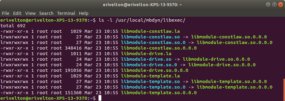
Now, it is time to create my own module. In order to do it, I first started by compiling the proposed modules to check if they worked well. These modules are: driver caller, constitutive law and element. I followed the wiki page and FAQ page to undesrtand better what they are and how to use them in the mbdyn code.

As can be seen in the following picture, the module was successfully built.

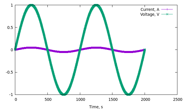
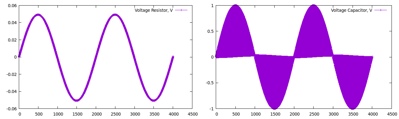
Next step was to create a MBdyn code to run the module instances as proposed in the entry test. However, I took some time prior to understand how those modules works and how I could implement them. So, I found other interesting module called fab-electric developed by Eduardo Okabe. I built it and ran some fundamental eletric circuit exercises:

• a power supply connected to a Resistor;
• a power supply connected to a Resistor-Capacitor circuit (RC circuit);

You can see the results in the following pictures. The first one shows the current and voltage in the resistor. The second one shows the voltage in the resistor and capacitor.

So far, this is what I have to present. I will continue developing my onw module soon and keep it updated here and in the GitLab page. In the mean time, I will also explore the project ideias.

Stay tuned !